My Gridcoin ‘Mining’ Journey So Far
Introduction
About a year ago I was looking into options to make a little extra money from my numerous computers sitting in my office. Bitcoin was no longer an option, due to the prevalence of mining through the use of specialized ASICs, meaning the dollar return from using a home PC wouldn’t even come close to covering the electricity costs.
It was during my search that I first stumbled across Gridcoin, an alternative cryptocurrency to the likes of Bitcoin. Gridcoin perfectly fit what I was looking for, I could donate my many computers idle time to contribute to scientific research projects run by universities and research organizations, by running software called BOINC, and get rewarded in an amount of Gridcoin relative to the amount of work my computers had completed.
There was a bit of a learning curve getting the software setup, and choosing the right projects to contribute to for my hardware, but the whole package appealed to my interest in building pc’s, optimizing for best results and not simply burning power on useless hashing to generate bitcoin (I know people say hashing is necessary to secure the Bitcoin blockchain, but to me that just means the Bitcoin’s core is extremely inefficient). Since starting with Gridcoin I have become even more convinced that this cryptocurrency can seriously encourage contribution to volunteer computing projects, as well as be viable stable currency that can hold it’s own against other top cryptocurrencies.
Important points for me:
- Gridcoin rewards are in return for contributing valuable compute resources to scientific research.
- Decentralization – Rewards are issued to researchers/miners by the distributed Gridcoin network, not an individual or group in control.
- Issue of rewards is secure, such that users cannot cheat the system to get more Gridcoin
- By contributing to Gridcoin and BOINC, and encouraging more people to contribute, this will draw more people into contributing their computers idle processing time to valuable scientific research and in turn the price should increase due to the fact that many people will never sell Gridcoin for less than the electricity cost to earn them.
- An active development team who have made fantastic progress in improving the Gridcoin software, along with an involved community of enthusiastic researchers/miners.
Growth Potential
The current market capitalization of Gridcoin is just below USD $60,000,000. There are currently 61 cryptocurrencies with a market cap above USD $500,000,000! Given the current state of Gridcoin user growth, the huge benefits to society of BOINC contribution, large existing BOINC user base, and the fact that almost any PC can take part earning Gridcoin, I strongly believe that in the short term Gridcoin will also be in this category, and it has potential to go much further in the mid to long term.

Gridcoin price for the last 90 days, approximately 500% increase!
At the time of writing (3 Jan 2018) there are almost 10,000 members signed up to pool mine through GRC Pool, and another 1800 actively solo mining (which is a bit more effort to get started). Just six months ago GRC Pool had only 2600 members (approximately). So there are already a lot of people involved contributing to Gridcoin, and the number is now growing quickly as more people become aware of it’s existence. It would be easy to say that the price increase above is just a temporary spike driven by speculative trading, however this increase in users is real organic growth which suggests otherwise.
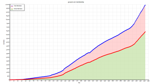
GRC Pools user numbers for the last 342 days
Gridcoin issues a target amount of 48,000 GRC per day, regardless of how many users are involved. So as more people get involved, the amount of Gridcoin each user receives on average will decline. Since the electricity consumption, and therefore cost of contribution is steady, this should (and history shows does) cause an increase in the value of the coin. My advice is don’t sell the Gridcoin you earn! It will be worth much more in the future!
Getting Started
If you want to get started contributing and earning Gridcoin, I recommend going to Gridcoin.Science, and follow the instructions to get set up in GRC Pool (link under ‘Get GRC -> Pool Mining).
I plan on writing some more articles in the coming weeks that will help demystify how to select projects to contribute to, give an idea of how much you will be rewarded, show some techniques to monitor multiple computers remotely, and give an overview of my setup.
Just remember, even by contributing your possibly humble pc resources you are helping contribute to some fantastic scientific projects and discoveries, and accumulate some Gridcoin at the same time before the price sky rockets. Thank you for reading!
Reference Information
https://Gridcoin.Science – A new Gridcoin Landing page with a lot of information on Gridcoin, and how to get started.
http://Gridcoin.us – The original Gridcoin landing page. (Gridcoin is not centralized, so there is no ‘official’ site 🙂
https://steemit.com/trending/gridcoin – Many community members post useful information on the Steem platform, and is worth checking regularly.
https://poloniex.com/exchange#btc_grc – An online exchange where you can check the value of Gridcoin against Bitcoin.
https://www.coingecko.com/en/price_charts/gridcoin-research/usd – A site with heaps of cryptocurrency info, take a look at the Gridcoin to USD price!
GWT/Javascript Cisco simulator for CCNA prep.
A while ago I experimented with writing a program to simulate the behaviour of Cisco switches and Routers, with the idea of embedding it in a webpage so that it could be accessed for free using any web browser. This application would need to be rather complex, and could have been quite processor intensive, so I chose to write the application using java as this could also be easily embedded in a webpage. Nowadays java is very unpopular for such purposes, and most web browsers impose restrictions on java applications which simply make it too hard for end users. I decided that for this program to be of any use I would need to find another method to allow this to run inside a web browser.
It seemed that the most compatible method would be to rewrite the program in javascript, but this was simply not an option due to the huge effort involved, and that I could not bear to even think about writing a large OO program in javascript. I soon stumbled across a development toolkit made by Google, called GWT (Google Web Toolkit). This was exactly what I needed! GWT allows code to be written in Java, and then compiled into javascript which can be used in a webpage.
In order to use GWT I did need to make some changes to the original program, mostly user interface related. One great thing with GWT is that it allowed me to use Eclipse for development, and also allows debugging which could be difficult if writing entirely in javascript.
You can check out this simulator at http://www.net-refresh.com.
Free Cisco CCNA Simulator
I have been working on this Cisco simulator for a good while now, aimed at helping people to familiarize themselves with the configuration of Cisco switches and Routers via the command line. This simulator is aimed primarily towards students who are preparing to sit their CCNA and ICND exams.
The motivation behind creating this simulator was due to my struggles with remembering all the different requirements in the CCNA syllabus. There is so much material to learn that I could study a topic and believe I had a good understanding, but after moving to another topic found I would quickly forget much of what I had learnt! I would also regularly use GNS3, an excellent free emulator for Cisco devices, but without a proper study plan I would inevitably miss certain essential topics.
This simulator has been programmed in java, so that it can be imbedded in a webpage with no need to download or install any software on your PC. I’m sure there will be no shortage of criticism for my choice of java, I feel it is very fit for the purpose. I am unable to imbed java on this site, but if you head across to www.net-refresh.com you will find a number of scenarios available for you to practice.
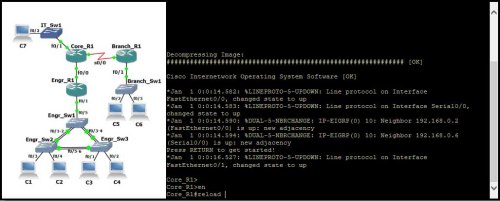
The CCNA simulator’s applet interface
If you choose from one of the practice scenarios here, you will be presented with an interface like the one above. Depending on your version of java and your security settings, the applet may not display. If this is the case, please follow the instructions here to enable java on this site.
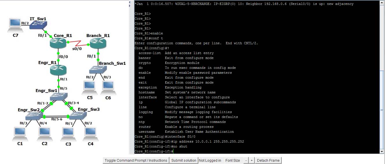
On the left hand side is a diagram of the network topology, and the right is the console area. You can select a device to configure by clicking it’s image on the left, and this is the equivalent of connecting a pc to the Router/Switches console port and opening a console connection. Commands can now be typed in the right to configure the device.
Each scenario has a set of instructions, which can be seen by clicking the ‘Toggle Command Prompt/Instructions’ button. As certain objectives are completed they be listed as such.
The ‘Detach Frame’ button allows the simulator to be separated from he browser window, although if the page is closed the applet will close also. In some browsers the simulator will not display correctly, in which case detaching the frame will be the best option.
This simulator is undergoing constant development, so more functionality is being added regularly. I hope you will check it out and find it useful!
Can cellphone towers affect Wifi Performance?

I have read quite a few posts in forums around the web, in which people are suspecting that a new cellular tower nearby may be the cause of their slow Wi-Fi performance. I could not however find any case where a solution had been found, so I will share an experience I have had with this.
Recently I was involved with trying to determine the cause of very low throughput on a number of Wi-Fi access points, providing coverage over a large outdoor area.
We were equipped with an Anritsu S332D Sitemaster, with spectrum analyzer, and after testing the antennas we had a look at the 2.4-2.5GHz spectrum in search of any sources of interference. The location was surrounded by 3 cellular towers, with the nearest being less than 100m away, so we suspected that there may be some interference in the 2.4GHz band due to intermodulation. Surprisingly the band was very quiet, and there were no signals that did not belong there.
Next we looked more closely at the cellular frequencies, the nearest of which was centered on 2.115GHz. To our surprise the level was much higher than expected, with our low gain, wideband antenna, the received power was -20dBm! This made us think that the high level cellular signal was swamping the access point’s front end receiver leading to receiver desensitization, but surely access points would have a pre filter before their sensitive receiver circuitry wouldn’t they? Well I can’t answer this for certain, but I have seen some application notes showing the first stage after the antenna being a Low Noise Amplifier. If this is the case I am not surprised that high power transmitters, even if they are out of band, will impact on the performance of Wi-Fi. I should say, the cell site does appear to be operating within their license.
In order to test this theory two band pass filters (which allow only the frequencies from 2.4GHz to 2.5GHz to pass and severely attenuate all others) were ordered and installed on the two antennas of one access point on site. These filters were able to attenuate the offending signal by 60dB. Throughput tests were carried out before and after the addition of the filters, and the improvement was clear. Before installation of the filters, performance at about 20m was down to about 1Mbps. After installation this jumped to above 30Mbps, and the engineer was able to get around 30Mbps to a distance of almost 100m.
We also visited some other locations near cell sites, and measured the levels there also. At most sites we received levels between -45dBm and -60dBm, and there were no reports of poor Wi-Fi performance (although no thorough throughput tests were carried out).
So if you have ruled out all other possible causes of your poor Wi-Fi performance, it is possible that a nearby cell site could be the cause of your problems (or lack of decent receive path pre-filtering depending on your angle). You will however need to get your hands on spectrum analyzer in order to determine this conclusively.
Ray Tracer Part Four – Shading and illumination
Shading and Illumination
So far we can intersect a ray with a sphere, and calculate the normal at the intersect point, and in this article we will extend the raytracer to shade the sphere. This will help give the illusion of depth to the sphere.
First it is necessary to check whether an intersectPoint is illuminated by a lightsource, or whether it is in shadow. This is achieved by casting a ray from the intersect point towards the lightsource, and testing whether it intercepts any objects. As soon as any object is intercepted, we know the intersectionPoint is in shade, and can stop testing. (note, although neither option is realistic, I have assumed a transparent object will not cast a shadow)
rayToLight = lightSourceCentre - intersectpoint;
lightSourceDistance = rayToLight.length();
rayToLight.normalise();

for(all non transparent objects in scene)
{
   if(currentObject.intersect(intersectPoint, rayToLight, lightSourceDistance, normal))
   {
      // ray hit an object CLOSER THAN LIGHTSOURCE
      // so point is in shadow
   }
}
This can be put in a method that returns true if a point is in shadow. Be sure to ensure that the ray intersects at a distance less than the light source distance.
Diffuse Illumination
First we will calculate the diffuse lighting component. This assumes that any light that hits the surface is scattered evenly in every direction. So regardless of the viewing angle, the point will appear to be the same color. The intensity of the light does however depend on the angle between the surface normal vector, and the vector towards the lightsource. If the surface is perpendicular to the light source vector, the surface will receive maximum illumination (and if parallel, the surface will receive no illumination). This diffuse lighting component can be calculated as follows:
intersectToLight = lightSourcePoint - intersectpoint;
intersectToLight.Normalise();
lDotNormal = surfaceNormal.Dot(intersectToLight);
lDotNormal = lDotNormal < 0 ? 0.0f : lDotNormal;
diffuseComponent = kd * surfaceColor * lightSourceColor * lDotNormal
‘kd’ is the diffuse coefficient, a value between 0 and 1. Both the surfaceNormal vector and vector towards the lightSource must be normalised, and lDotNormal must be checked to ensure the value is greater than 0. We know of course that if the dot product is negative then the surface is facing away from the lightsource, and is thus in shadow.
Phong lighting
The next component to calculate is the specular component, in this case Phong. This gives an object the appearance of being shiny, such as plastic or metal. Again, the specular component is only calculated if the lDotNormal value is positive.
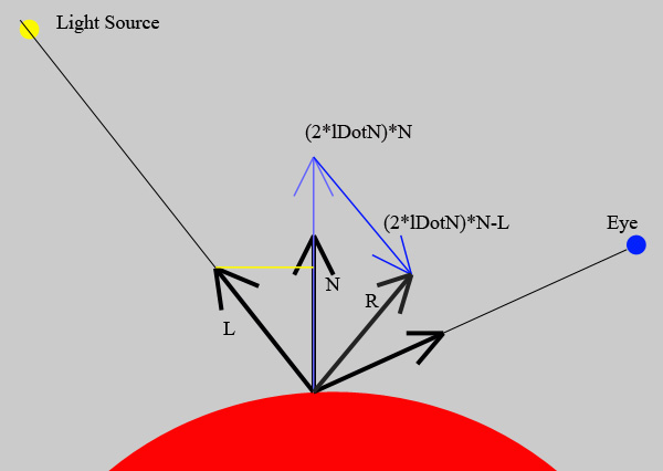
To begin with we know the vector L, N, and V (vector towards the eyePoint), and we want to find the vector R (R is the same as the reflection vector, which will be needed later). First, ensure L, N and V are all normalised. Referring to the image above, the vector R can be calculated as (2*lDotN)*N – L. Next take the dot product of R and V. this RdotV value is then raised to the power ‘n’. This n value determines how concentrated the specular highlight will be. A large n value will lead to a smaller spot, a smaller n value will result in a broader spot. We also have another value to adjust, the specular constant ks. This should take a value between 0 and 1, and can be used to scale the intensity of the highlight.
Phong Component = ks*lightSourceColor*(RDotV^n)
This will give the specular highlight the same color as the light source color. If the objects material is metallic, such as gold, the specular component (and reflections) tend to take on the color of the material. Thus for metallic surfaces the Phong component becomes:
Phong Component = ks*lightSourceColor*surfaceColor*(RDotV^n)
Ambient Lighting
Ambient lighting is the addition of some lighting to every intersection point, even if in shadow. Without this surfaces in shadow would appear completely black, which gives very unrealistic images. Adding ambient lighting like this is far from realistic, but is simple to apply. The way in which i have applied it is to calculate it for every light source in a scene, dependent on the lightsources colors (ka is an ambient constant, I use 0.1).
Ambient Component = ka * kd * lightSourceColor * surfaceColor
The total illumination for a point is the sum of all these components.
Total Illumination = Diffuse + Specular + Ambient
Modifications
An alternative to Phong illumination is Blinn-Phong. Blinn-Phong has the advantage that it is faster to compute than Phong, with almost the same effect.
In the diffuse illumination formula, distance from the light source does not effect the intensity of illumination. An object close to the light source, and one very far away will receive the same illumination (provided the angle between their normals and the lightSource ray are the same). If you would like to account for this, simply divide the total illumination by (distanceToLightSource^2).
Using point light sources casts very hard shadows, by using soft shadows the realism of images can be greatly improved. In order to cast soft shadows we instead use area light sources, and cast many shadow test rays from each intersection point towards random points on the surface of the area light source. The ratio of obstructed to unobstructed rays then determines how much illumination is applied to the surface point.
Ray Tracer Part Six – Depth Of Field
Depth Of Field
Adding depth of field capability to your ray tracer is well worth the effort, and you’ll be pleased t know that it is not all too difficult either. You will however need to wait significantly longer for your images to render, as every pixel now needs to send multiple rays in order reduce noise.
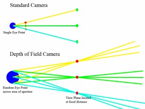
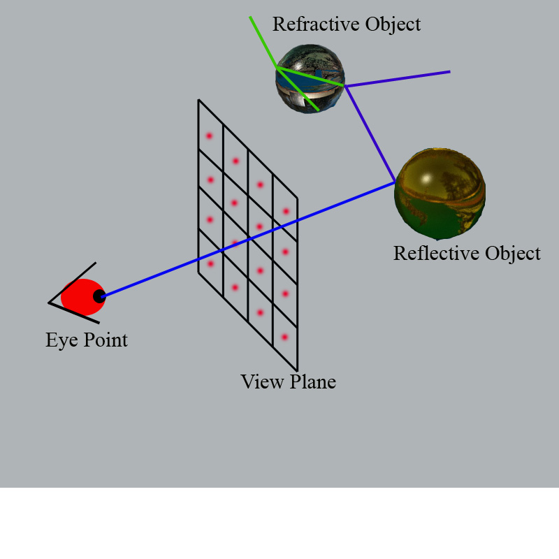
The illustration below gives a basic idea of how we can achieve this effect. For simplicity lets assume 2 dimensions, and only 3 pixels need rendering. The standard camera will cast one ray ( yellow, green, cyan) for each pixel, from the eye point through the associated view plane point. In the case of DOF camera, multiple rays will be cast for each pixel. This time however the view plane will be situated at the desired focal distance, and the eye point will be randomised around the eyepoint, to an extent dependent on the radius of the aperture.
So implementing this in code should be fairly easy. The approach I will describe requires recalculating the same parameters as for the standard camera, but this time the view plane is located at the focal distance. Whenever the Focal distance is changed, these parameters will need to be recalculated.
The changes that need to be made to the standard camera code are as follows:
Calculate the focal distance, assuming the focus should be set to the lookat point.
Focal Distance = Length(lookAtPoint – eyePoint)
If the focal distance is instead set at some other value, calculate a new point at the centre of the new view plane.
Calculate the new half width of the view plane.
halfWidth = focalDistance *tan(fov/2)
So now the bottomLeft , and increment vectors will be calculated correctly using the same code as for the standard camera.
In order to randomise the eye point later, 2 vectors will also be precalculated, such that we can add them to the eye point.
  xApertureRadius = u.normalise()*apertureRadius
  yApertureRadius = v.normalise()*apertureRadius;
Now we need to change the code in the getRay method.
Random rays work well, so we can generate 2 random numbers,
One for the x variation around the eyePoint, and one for the y. I don’t believe the extra computation to ensure the new eye points lay inside a circular aperture make much difference, however you can decide.
  R1 = random value between -1 and 1
  R2 = random value between -1 and 1
  ViewPlanePoint = bottomLeft + x*xInc + y*yInc
  newRandomisedEyePoint = eyePoint+ R1*xApertureRadius + R2*yApertureRadius
  ray = (ViewPlanePoint - newRandomisedEyePoint).normalise()
Now everything required to generate an image with depth of field is complete. Instead of firing just a single ray through each pixel, we now add something like the pseudo-code below.
  Color tempColor(0.0f,0.0f,0.0f);
  for(int i = 0; i < numDOFRaysPerPixel; i++){
      camera.getRay(x,y, castRay, eyePoint);  // where castRay and eyePoint are references and set by the getRay method
      tempColor.setBlack();
      traceRay(eyePoint, castRay , tempColor....);  //tempColor will be set to the resulting color for this ray
      displayBuffer.add(x, y, tempColor); // add all the DOF rays to the same screen pixel
  }
  displayBuffer.divide(x,y, numDOFRaysPerPixel);  // divide the pixel by the number of DOF rays cast
This will cast the same number of DOF rays for every pixel in the screen, which is not very efficient. Consider these two situations. First where there is an object situated on the focal plane (in the path of our ray), and secondly where the object is situated far behind the focal plane. In the first case all our depth of field rays will converge to the same point, so casting a large number of rays is wasteful. In the second case, many more rays will be required, as each ray will ‘pick up’ colours form points which are very far apart, and possibly intersecting different objects (refer to the figure above). So instead of casting a fixed number of DOF rays per pixel an improvement can be made by continuing to cast rays until a certain error condition is met. For example once the effect on the final colour of a pixel by additional DOF rays is less than a defined limit.
Ray Tracer Part Three – Adding a Sphere
Now lets create something to add to our scene. One of the simplest objects we can add is a sphere, so lets get started with that first. We can define a sphere in our world as having a position, and a radius. But first lets create an abstract Object class, that all objects can derive from.
Object Class
Every object in our scene will share some common properties. They will all have a color, and they will all have properties related to how they are illuminated. They will also all need an intersect method. In C++ the basic Object class would look something like the code below:
class Object {
public:
    Color color;
    float kd; // diffuse coefficient
    float ks; // specular coefficient
    float pr; // reflectvity
    float n;  // phong shininess
    float IOR; // index of refraction
    Object(Color color, float kd, float pr, float ks, float n, float IOR, bool transparent){
        ..... set the attributes
    }
    virtual int intersect(Point &origin, Ray &ray, float &distance, Ray &normal) = 0;
}
In the intersect method, the ‘distance’ reference contains the closest intersect distance thus far, and if the object being tested is intersected closer than this, distance will be modified;
Sphere Class
The sphere class thus needs to provide an implementation of the intersect method. The following formula can be used to determine if a ray intersects a sphere, and the distance of the hit.
A*(distance^2) +B*distance + C = 0;
where
A = castRay.Dot(castRay)
B = 2*(origin - sphereCentre).Dot(castRay)
C = (origin-castRay).Dot(origin-castRay) - radius^2
This is a quadratic equation, so the two solutions for the intersect distance can be obtained using the quadratic formula.
When we test a ray we want to consider 3 possible situations.
1) The ray misses the sphere – When the discriminant is less than zero. or the intersect distance is greater than that of an intersect test with another object
2) The ray hits the sphere from the outside – When the discriminant is greater than zero, and the two calculated intersect distances are positive.
3) The ray hits the sphere from the inside – When the discriminant is greater than zero, and the lower distance is negative.
A = ray.Dot(ray);
originToCentreRay =  originOfRay - centreOfSphere;
B = originToCentreRay.Dot(ray)*2;
C = originToCentreRay.Dot(originToCentreRay) - radius*radius;

discriminant = B*B -4*A*C;
if(discriminant > 0){
   discriminant = std::sqrtf(discriminant);
   float distance1 = (-B - discriminant)/(2*A);
   float distance2 = (-B + discriminant)/(2*A);
   if(distance2 > FLT_EPSILON) //allow for rounding
   {
      if(distance1 < FLT_EPSILON) // allow for rounding
      {
         if(distance2 < distance)
         {
            distance = distance2;
            normal.x = 10000;
            return -1; // In Object

         }
      }
      else
      {
         if(distance1 < distance)
         {
            normal.x = 10000;
            distance = distance1;
            return 1;
         }
      }
   }
}// Ray Misses
return 0;
You will notice that first the discriminant is checked to ensure it is greater than zero. If the discriminat is negative the ray does not intercept the sphere. If the lesser of the two intersections is negative and the greater distance is positive, then the origin is inside the sphere. A value of -1 is returned here as it is useful for correcting the normal later. It is also necesary to ensure that this intersection is closer than any previous object intersection.
The normal.x value has been set here to an arbitrarily large number, so that other code knows it needs to explicitly calculate the normal. Of course the normal vector could be calculated simply here, however I found a slight performance improvement by only calculating the normal once we know of the nearest object.
Normal vector
In order to calculate lighting, reflection and refraction rays, we need to know the normal vector at the point of intersection. All objects will need this method, so lets add it to the Object abstract class.
virtual void getNormal(Point& intersectPoint, Ray& normal) = 0;
In the sphere class, this will look something like this
void getNormal(Point& intersectpoint, Ray& normal)
{
   normal = intersectPoint - sphereCentre;
   normal.Normalise();
}
That’s it, now we’re ready to move on to applying illumination and shading to the sphere.
Ray Tracer Part Two – Creating the Camera
The camera is responsible for creating a ray which passes from they eye point through the pixel we want to render.
The camera will be defined by an ‘eye point’, a ‘look at point’, and a ‘field of view’. It is also necessary to define an ‘up vector’ for the camera, however this will be assumed to be always up in this case (0,1,0).
When a camera is constructed, several attributes will be set which will allow the easy generation of rays later. The first parameter we will calculate is the Point located at the bottom left of the view plane. We will then calculate two vectors, one which will be added to the bottom left point for every increase in x on the view plane, and one which will be added to the bottom left point for every increase in y on the view plane.
Constructing the camera
Our constructor requirements,
Camera(Point eyePoint, Point lookAtPoint, float fov, unsigned int xResolution, unsigned int yResolution)
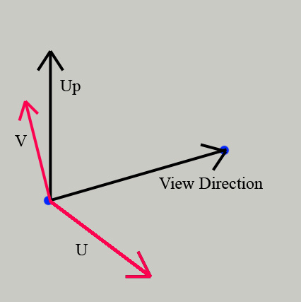
First calculate the “viewDirection” vector.
viewDirection = lookAtPoint - eyePoint;
Next calculate the V vector , here we will assume up = (0,1,0).
U = viewDirection x up
Now recalculate the up vector, (if the camera is tilted, the cameras up vector will not be (0,1,0), right?)
V = U x viewDirection
Be sure to normalise the U and V vectors at this point
Obtaining the bottom left point on the viewplane is now easy.
viewPlaneHalfWidth= tan(fieldOfView/2)
aspectRatio = yResolution/xResolution
viewPlaneHalfHeight = aspectRatio*viewPlaneHalfWidth
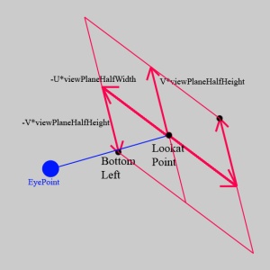 viewPlaneBottomLeftPoint = lookatPoint- V*viewPlaneHalfHeight - U*viewPlaneHalfWidth

So now we need the increment vectors, which will be added to the bottomLeftViewPlanePoint to give our viewplane coordiantes for each pixel.
xIncVector = (U*2*halfWidth)/xResolution;
yIncVector = (V*2*halfHeight)/yResolution;
Getting a ray
Now we want a method that can return a ray that passes from the eye point through any pixel on the viewplane. This can be easily obtained by calculating the view plane point, and then subtracting eye point. x and y are the viewplane coordinates of the pixel we want to render, numbering from the bottom left.
viewPlanePoint = viewPlaneBottomLeftPoint + x*xIncVector + y*yIncVector
castRay = viewPlanePoint - eyePoint;
Conclusion
This is by know means the only way to create a camera, but is fairly intuitive to get started. It is also easily modified at a later date to allow the calculation of anti-aliasing rays.
Next – Adding a Sphere
Ray Tracer Part One – What is Raytracing?
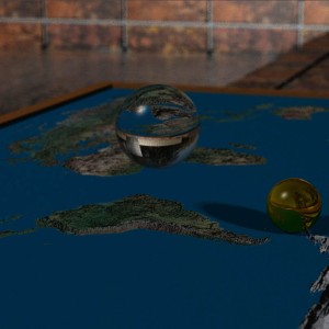
The following image was generated by a raytracer I have written in C++. I originally wrote this as a programming assignment for a course at Canterbury University, COSC363 – Computer Graphics. The program can be downloaded from this page.
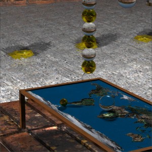
This render illustrates many of the features currently implemented. Supported object types are spheres, cones, boxes, and surfaces, these objects can be made reflective or refractive, and have textures applied to add realism. Area light sources allow soft shadows to be cast. Surfaces can be bump mapped, giving the impression of an irregular surface (or water surface with refraction) , or even used to create a complex 3D surface. A depth of field camera can also be used, to bring objects at a certain distance into focus, while leaving others blurry. An environment map can be used to surround the scene, and fill in that dead space, and makes reflections look much more realistic. A KD-tree is used to speed up the raytracing process when a large number of objects is added. Photon Mapping is also supported, allowing caustic lighting with refractive objects.
The basic idea
Raytracing generates an image by tracing the path of light from an eye point, through each pixel of an image, and coloring each pixel depending on the objects the ray intercepts in it’s path. When a ray hits an object, the color contribution of that hit is calculated (depending on material properties, and lighting…) and if the material is reflective or refractive, additional rays are calculated and traced until a certain end condition is met. When a ray hits a reflective object a reflective ray is generated. When a ray hits a transparent object two rays must be generated; a reflective ray and a transmission ray.
The basic raytracing algorithm
Probably the easiest way to implement a raytracer is by using recursion. The following pseudocode is not supposed to be in anyway complete or concise, but is rather intended to provide a simple introduction to the idea.
Render(){
   for each pixel in image {
      viewRayOrigin = eyePoint;
      viewRay       = currentPixelLocation - eyePoint;
      maxRecursiveDepth = 7; // or more
      traceRay(viewRayOrigin, viewRay, currentPixelColor, maxRecursiveDepth)
   }
}

traceRay(origin, viewRay, pixelColor, depth){
  if(depth <= 0) // our end condition
     return;

  nearestObject = getNearestIntersection(origin, viewRay, interceptDistance);

  interceptPoint = origin + viewRay*interceptDistance;
  pixelColor += calculateLighting(nearestObject, interceptPoint);

  if(nearestObject is transparent){
     transmissionRay = getTransmissionRay(....);
     traceRay(interceptPoint, transmissionRay, pixelColor, depth-1);
  }

  if(nearestObject is reflective or is transparent){
    reflectiveRay = getReflectiveRay(...);
    traceRay(interceptPoint, reflectiveRay, pixelColor,depth-1);
  }
}
Now obviously many details have been left out from this, and as you develop your code you will undoubtedly encounter undesired visual artifacts at some point.
If you are new to computer graphics or ray tracing, some of these terms may be new to you, but it is my intention to introduce these topics in an easy to digest manner, and provide an explanation of how these features can be implemeted so hopefully you too can create a working ray tracer. Ray tracing is very computationally expensive, so consider this when deciding which language to use.
